sardine-track — the story
Why This Exists
It’s easy to gaslight yourself into thinking you’re having panic attacks and are lazy. Sometimes people have panic attacks and are lazy, and that’s entirely normal.
But when the shortness of breath is uncoupled from emotion, when the “laziness” is less sloth and more that you’re stuck in a quagmire of quicksand despite wanting to do so much - there’s something making your body react that way.
The sun was making me sick.
At least that was my intuition, but that seemed insane. I had low vitamin D for years and was told to get more sun. But like clockwork, high UV index days would leave me sick the next day, or two, or three. A sunburn put me in bed for a week with what felt like the flu.
I figured I was just getting older. Also, I’m hella pale, maybe this was a white people thing no one had mentioned to me.
Though coupled with a family history sprinkled with, and a genetic profile loaded for, SARDs and autoimmune disease associated mutations - I decided to quantify it. It became painfully clear to me by the data, that unfortunately, the sun has been making me sick.
That’s why I started a spreadsheet, but it was useless in clinic, rows upon rows of color-coded entries with no succinct way to visually communicate what they meant in a 15-minute appointment. While exhausted and in pain and anxious about being dismissed again, trying to recall the practice conversation I had with an imaginary clinician explaining what was going on.
After 90+ days I gave up. I got depressed. I kept getting sick. My sick leave was running dry at work, and without a diagnosis I didn’t feel confident that I could get FMLA protection. (Note: This also accounts for the 127 day logging gap in my data.)
Then I picked it back up. I can’t remember exactly what the impetus was - probably another rheumatologist doubting me while ER doctors were writing “I believe her condition to be rheumatic in nature.” Meanwhile my dermatologist was doing her damnedest to get the best biopsy shave for DIF this side of the Mississippi. Pretty much the size of a mercury dime.
Claude Sonnet (and later Opus) helped me build it. I’m not a strong coder, I can get around, and I know how to make infinity while loops, but I’m far from skilled. The LLM assisted me in building the stack, troubleshooting bugs, and providing the kind of cognitive support I could direct, debug, and reiterate. And if Claude can be annoyed, I most certainly annoy that poor tireless machine.
Throughout all of this, I was in and out of doctors appointments and a few ER visits, and eventually arrived at a confirming “cool, I was right” / “fuck, why do I have to be right about this?” diagnosis. Eight months from when I started aggressively seeking treatment to confirmed diagnosis, albeit nearly 9 years from the onset of symptoms. I beat the odds, the average diagnostic delay is four to seven years after aggressively pursuing answers. I’m lucky. A lot of people aren’t.
My current diagnosis is acute cutaneous lupus erythematosus which is also understood to be systemic lupus erythematosus, confirmed by biopsy and with woefully unremarkable serology. But autoimmune disease evolves, and we are constantly learning new things about the human body. The differential will shift. The ICD codes may change. Whether we end up calling it lupus or the Hokey Pokey Disease, getting that process started - having longitudinal evidence, having dates, having correlations - matters enormously for health outcomes down the road.
This tool isn’t a lupus tracker necessarily, though it is designed around an evolving case of predictably photosensitive lupus. It’s a tool developed to help spot patterns that may otherwise remain as hunches without quantification, the intent is you can change it to fit your case. Whatever you’ve got going on.
Philosophy
Patients are experts on changes in their own bodies. You know when something is wrong, even when tests are “normal.” You also probably, for the most part, know the difference between normal and “oh no this is no good now.” Trust that instinct.
Correlation is worth investigating, even when causation isn’t proven. If UV exposure consistently precedes your symptoms, that pattern matters - regardless of whether a doctor believes you yet. Or hell, you don’t believe you yet.
Your data is yours. No surveillance, no selling, no cloud lock-in. You can delete everything and walk away at any time. We are all volunteers here.
Invisible illness deserves visible evidence. When your symptoms are dismissed as anxiety or “borderline,” a longitudinal graph can shift the conversation. It can also help you recognize patterns and symptoms you may have normalized.
Diagnostic complexity is real. Some conditions take years to name. The average diagnostic delay for lupus alone is four to seven years, and it isn’t even a particularly rare disease, merely uncommon. Tools like this exist to help you survive that journey and shorten it where and when possible. This is meant to help both the patient and practitioner, so that you can both be on the same page and communicate in one another’s jargon effectively enough to figure out what the right questions to be asking are.
Acknowledgments
Built by C. Alaric Moore, a USPS technician, mechanic, and patient who got tired of being told that there weren’t any answers or that every symptom was independent of the other.
Assisted by Claude (Anthropic) across multiple model generations and roles. Sonnet handled the original build. Opus (nicknamed Clode) led the forecasting-model work, data analysis pipeline, and the /interventions rebuild. A second Claude instance (Wolf) handles statistical validation and clinical-literature cross-checking for features that could otherwise drift into confirmation bias. A third instance (Claude-Work) covers brainstorming. H/t to GitHub Copilot for closing parentheses and other surprisingly convenient features.
The app’s model explainer and much of this narrative were written collaboratively — where the voice is right, it’s because a tireless language model internalized the tone after many, many iterations.
Inspired by an unending need to make everything useful, even illness, as well as a low tolerance for hand-waved diagnostics and anchoring bias.
How the forecasting model works — MODEL.md
Flare Prediction Model
A transparent, statistical model for predicting lupus flare risk from daily observations. No black box — you can see exactly how every prediction is made, and tune it yourself.
How It Works
Each day, the model computes a flare risk score (0-25) by summing weighted contributions from multiple input categories. A score at or above the threshold (default 8.0) is a predicted flare.
Before scoring, each observation is enriched with multi-day context via _inject_scoring_context(), which pre-computes rolling metrics that span multiple days. This means the model isn’t just looking at today — it’s looking at patterns building over the past 1-3 weeks.
Scoring Categories
1. UV Dose
UV exposure is the strongest environmental predictor (Cohen’s d = +1.29, p < 0.0001 for 3-day cumulative sun exposure).
The dose is computed as an interaction: (weighted_UV_index ^ 1.5) x sun_exposure_minutes x protection_factor. This captures that 30 minutes at UV index 10 is much worse than 30 minutes at UV index 3.
| Condition | Points |
|---|---|
| UV dose >= 800 | +3.0 x uv_weight |
| UV dose >= 400 | +1.25 x uv_weight |
| 4-day cumulative UV >= 2500 | +1.5 x uv_weight |
| 4-day cumulative UV >= 1500 | +0.75 x uv_weight |
The cumulative UV load uses a decay-weighted sum of the prior 4 days (yesterday 0.8x, 2 days ago 0.6x, 3 days ago 0.4x, 4 days ago 0.2x). Personal data analysis showed UV signal persists 2-4 days before major flares — unprotected ≥60 min exposure on day -1 fires on 79% of major flares vs 35% of non-flare baseline, dropping to 58% at day -4 (still well above baseline). The older 3-day window with 0.7/0.4/0.2 decay dropped off too aggressively for a signal that stays visible this long. UV lag analysis shows 24-hour lag has the strongest single-day flare correlation.
Protection factors: none (1.0), SPF + hat (0.3), full cover (0.1), indoors only (0.0).
2. Physical Overexertion
Steps relative to personal baseline, adjusted for sleep.
| Condition | Points |
|---|---|
| Overexertion ratio >= 1.8 | +2.0 x exertion_weight |
| Overexertion ratio >= 1.4 | +1.5 x exertion_weight |
Overexertion = (steps / personal_step_baseline) x (8 / hours_slept). Falls back to raw steps/hours ratio if no baseline is set.
3. Basal Temperature Delta
Deviation from personal temperature baseline in Fahrenheit.
| Condition | Points |
|---|---|
| Delta >= 0.8 F | +3.0 x temperature_weight |
| Delta >= 0.5 F | +2.0 x temperature_weight |
| Delta >= 0.3 F | +1.0 x temperature_weight |
4. Individual Symptoms
Each symptom category is a binary flag (present/absent) with its own weight:
| Symptom | Weight | Notes |
|---|---|---|
| Neurological | 1.5 | Numbness, tingling, vision changes |
| Cognitive | 1.0 | Brain fog, memory, word recall |
| Musculature | 1.5 | Muscle pain, cramping, weakness |
| Migraine | 1.0 | Headaches, light sensitivity |
| Pulmonary | 1.0 | Air hunger, chest discomfort |
| Dermatological | 0.75 | Rash, photosensitivity |
| Mucosal | 0.25 | Dry mouth, dry eyes |
| Rheumatic | 0.5 base | Joint pain without specificity |
| — major joints | 2.0 | Hip, knee, shoulder, elbow, ankle, wrist, jaw |
| — minor joints | 1.0 | Finger, toe, hand |
Rheumatic scoring parses the notes field for joint names to differentiate severity.
5. Pain & Fatigue
Pain and fatigue are the strongest single-day predictors in this dataset (Cohen’s d = +1.01 and +0.83 respectively vs non-flare baseline). The previous cliff-at-7 threshold only fired on 12-25% of flare days; the laddered version below captures the full discrimination curve — pain >= 4 already separates flare days (75% hit) from non-flare days (5% hit).
| Condition | Points |
|---|---|
| Pain scale >= 7 | +3.5 x pain_fatigue_weight |
| Pain scale >= 6 | +2.5 x pain_fatigue_weight |
| Pain scale >= 5 | +1.5 x pain_fatigue_weight |
| Pain scale >= 4 | +0.5 x pain_fatigue_weight |
| Fatigue >= 7 | +3.5 x pain_fatigue_weight |
| Fatigue >= 6 | +2.5 x pain_fatigue_weight |
| Fatigue >= 5 | +1.5 x pain_fatigue_weight |
| Fatigue >= 4 | +0.5 x pain_fatigue_weight |
| Emotional state <= 4 | +2.0 x pain_fatigue_weight |
6. Symptom Burden Delta
The strongest predictor in the model. Raw symptom count saturates when you have chronic daily symptoms (e.g., neurological 76% of days, rheumatic 82%, dermatological 62%). What predicts a flare isn’t having symptoms — it’s having more than your usual number of them.
Computation:
- Recent: Mean daily symptom count over days -1, -2, -3
- Baseline: Mean daily symptom count over days -17 through -3 (14-day window)
- Delta = recent - baseline
The gap between the acute window (days -1 to -3) and the baseline window (days -3 to -17) is critical. Without it, the 3-day pre-flare symptom ramp bleeds into the baseline and dulls the signal.
| Condition | Points |
|---|---|
| Delta >= 3.0 | +3.0 x symptom_burden_weight |
| Delta >= 2.0 | +2.0 x symptom_burden_weight |
| Delta >= 1.0 | +1.0 x symptom_burden_weight |
Falls back to 0 contribution with fewer than 7 days of baseline history.
7. RMSSD Baseline Deviation
Data-quality correction (2026-06-14). Every RMSSD statistic in §7 and §7b below was computed from data corrupted by a bug in the iOS sync’s
queryRMSSD, which pooled inter-beat intervals across separate overnight HeartbeatSeries and applied no ectopic filter — inflating RMSSD up to 468 ms while same-day SDNN read ~12 ms. Fixed 2026-06-14 (per-series RMSSD + Malik 20% filter + median), and the prior ~365 days were re-backfilled from raw HealthKit. Treat the pre-correction numbers below — the ~105 ms non-flare baseline, the §7b pre-flare “oscillation”, the 2026-02-24 “164 ms anomaly”, and the tuned 1.25 personal weight — as superseded. The clean baseline (recent median ~24 ms) now matches Poliwczak’s 23.5 ± 10.0 ms below, which the inflated 105 ms never did. Provisional clean-data re-validation is in the box at the end of §7b.
Based on the cholinergic anti-inflammatory pathway: the vagus nerve tonically suppresses systemic inflammation. RMSSD (root mean square of successive differences in heartbeat intervals) is the best time-domain proxy for vagal tone. If vagal tone drops, the cholinergic brake weakens, and inflammation runs hotter.
Literature anchors. Thanou et al. 2016 (n=53 SLE patients, 505 visit pairs) found ΔRMSSD inversely correlated with ΔSLEDAI within subject (p=0.007) and LF/HF ratio associated with the SELENA-SLEDAI Flare Index (p=0.008) — direct evidence that RMSSD tracks lupus disease activity longitudinally. Poliwczak et al. 2017 (24-hour Holter, 26 SLE women vs 30 controls) confirmed SLE patients have chronically reduced r-MSSD (23.5 ± 10.0 ms vs 35.7 ± 16.3 ms, p=0.002), so baseline parasympathetic impairment is expected in SLE even between flares.
Computation:
- Recent: 7-day rolling average of nightly RMSSD (days -1 through -7)
- Baseline: 30-day rolling average (days -8 through -37, avoids overlap)
- Deviation =
(recent - baseline) / baseline x 100
| Condition | Points |
|---|---|
| Deviation <= -25% | +1.5 x rmssd_deviation_weight |
| Deviation <= -15% | +0.75 x rmssd_deviation_weight |
Personal data (post-bugfix rerun, n=26 flare clusters: 8 major/ER, 8 minor, 10 unspecified):
- Non-flare baseline RMSSD: ~105 ms (arithmetic mean), ~66 ms (geometric mean) — superseded (contaminated); clean baseline ~30–50 ms, recent median ~24 ms.
- On flare day, majors/ER drop robustly per-event. 7 of 8 events fall below baseline — day-0 arithmetic mean 42 ms (-60% vs baseline), median 20 ms (-81%). Wilcoxon signed-rank of per-event %drops vs 0: p=0.023. The one exception (2026-02-24 ER, RMSSD 164 ms / +56%) is a candidate data anomaly worth a sensor check. — confirmed 2026-06-14: this was the
queryRMSSDaggregation bug, not a sensor glitch. - Minors are noisy per-event. Only 5 of 8 drop; the other 3 show +70% to +150% rises. Arithmetic mean drop -28%, Wilcoxon p=0.38. Minor-flare detection relies more on the instability metric (section 7b) and respiratory rate (section 8) than on the level-based rule here.
- Aggregating across severities dilutes the major signal. All-flare day-0 mean drop is only -30% (Wilcoxon p=0.06) because unspecified events contribute a mix of rises and falls; the majors-only number is the one that matches Thanou 2016.
- Pre-flare day-1/-2 Cohen’s d vs non-flare baseline: -0.28 all flares, -0.18 majors alone, -0.37 minors.
- Mann-Whitney day-1 vs day-0 p=0.28 for majors, 0.32 all-flare — underpowered at current n, but the per-event signed-rank test on majors’ flare-day drops does reach significance.
Interpretation: Thanou’s longitudinal ΔRMSSD-ΔSLEDAI relationship reproduces in this single-patient dataset for major events specifically — the level-based rule in section 7 is carrying the majors, not the minors. The within-patient trajectory — decline into a flare, partial recovery after — matches the literature for majors; minor events require the instability and respiratory-rate features to catch.
Default weight is a conservative 0.5. Alaric’s personal weight is currently tuned to 1.25 based on observed performance (forecast accuracy view showed positive lift on caught vs missed flares). — superseded: tuned on contaminated data. Clean-data re-validation (§7b box) suggests deviation is the weaker of the two RMSSD features here (fires in 52% of quiet windows); pending re-tune on corrected data. Apple Watch RMSSD has ~29% measurement error vs chest strap (MAPE), but tracks relative within-person changes adequately for this purpose.
Returns no contribution with fewer than 4 values in either window.
7b. RMSSD Instability (Day-to-Day |Δ|)
Captures autonomic chaos rather than level-based withdrawal. Independent signal from section 7 — level-based deviation measures where RMSSD sits, instability measures how much it’s swinging; both can fire on the same day when the trajectory is collapsing chaotically. The two features are additive in scoring.
Superseded (2026-06-14) — the “oscillation” described in this paragraph is now known to be the cross-series aggregation artifact, not physiology: on corrected data, clean day-to-day |ΔRMSSD| transitions average ~8 ms, not ~120 ms. Retained for the record; see the re-validation box below.
Prototyped from the post-bugfix rerun analysis (rmssd_flare_rerun.py in the project root, generating rmssd_flare_rerun.png). That analysis, stratified by severity at n=26 flare clusters, showed that in the week before major flares RMSSD oscillates wildly — surging at day -6 (~100 ms), crashing at day -4/-3 (~50-60 ms), rebounding at day -2 (~85 ms), then collapsing on flare day (~45 ms). Mean day-to-day |ΔRMSSD| at the day-1 → day-0 transition reached ~120 ms in majors vs ~60-70 ms in minors and non-flare transitions. Crucially, the oscillation is a major-flare-specific phenomenon; minor flares show flatter trajectories, which is why the older aggregated analysis (n=21, not split by severity) showed a weaker pattern.
Computation:
- Recent: mean of |RMSSD[d] - RMSSD[d-1]| across days -1 through -5 (yields up to 4 adjacent-day deltas)
- Baseline: same metric across days -6 through -35 (~29 deltas — large window dilutes post-flare steroid oscillation days)
- Deviation =
(recent_mean - baseline_mean) / baseline_mean x 100
| Condition | Points |
|---|---|
| Deviation >= 50% | +1.5 x rmssd_instability_weight |
| Deviation >= 25% | +0.75 x rmssd_instability_weight |
Conservative default weight (0.5) pending validation. Requires >=3 recent deltas and >=10 baseline deltas to compute.
Clean-data re-validation (provisional, 2026-06-14, N=6 — underpowered). After the data-quality correction, a pre-onset-window analysis — did the feature fire in the 3 days before a major flare that had a clean (non-flare) run-up, vs matched quiet windows — on the corrected data found:
- Instability: fired before 4/6 (67%) of clean major onsets vs 31% of quiet windows — a ~2× pre-flare enrichment. This reverses an interim “instability is artifact” read, which was itself an artifact of the contaminated data.
- Deviation (§7): fired before only 1/6 (17%) of onsets but in 52% of quiet windows — poor specificity (RMSSD sits below its 30-day baseline more than half the time, consistent with chronic parasympathetic suppression), so the −15% threshold rarely discriminates.
Only 6 majors had a clean non-flare 3-day run-up (most arrive in clusters), so this is suggestive, not conclusive. Both weights left at 0.5 pending more clean flare events.
8. Respiratory Rate Baseline Deviation
Literature motivation (non-lupus-specific). Barfod et al. 2017 (Scandinavian Journal of Trauma, Resuscitation and Emergency Medicine, n=15,724 ED triage cohort) reported OR=1.15 per breath/min increase for ICU admission or in-hospital mortality within the subsequent two days. Michard & Saugel (2025) describe vital-sign drift as a marker of impending adverse events hours in advance. These are general critical-care deterioration findings, not lupus-specific. No paper in the Thanou/Poliwczak literature trail measured respiratory rate as a flare predictor; this feature is a mechanistic extrapolation from sepsis/deterioration to autoimmune flare.
Computation:
- Recent: 3-day rolling average of respiratory rate (days -1 through -3) — shorter window than RMSSD because the hypothesis is a 1-3 day signal
- Baseline: 14-day rolling average (days -4 through -17, gap avoids pre-event contamination)
- Deviation =
(recent - baseline) / baseline x 100
| Condition | Points |
|---|---|
| Deviation >= 15% | +1.5 x resp_rate_deviation_weight |
| Deviation >= 10% | +0.75 x resp_rate_deviation_weight |
15% above baseline is approximately 2-3 extra breaths/min for a typical resting rate of 16 breaths/min, consistent with the literature’s 3 breath/min difference between deterioration and control groups.
Personal data status — honest caveat. In Alaric’s dataset, comparing raw pre-flare rates cross-sectionally to non-flare rates gives a weakly negative Cohen’s d (-0.18 for majors, -0.16 all flares) — meaning her pre-flare respiratory rate sits slightly lower than her non-flare rate, the opposite direction of what the ICU literature predicts. That undermines the simple “elevated rate before deterioration” framing.
The feature nevertheless scores within-person deviation (3-day recent vs 14-day baseline) rather than cross-sectional group means, so a signal that only fires on specific days when her rate spikes above her own baseline could still be predictive. Her resp rate range is also narrow (~19-20 breaths/min, stdev ~1.5), so small absolute changes produce meaningful percent deviations — the feature is mechanically testable even if the group-mean signal is absent.
Live validation: the /model dashboard’s respiratory rate deviation chart (third card in the multi-day predictor panel) renders this deviation over time with dashed reference lines at +10% and +15% — the two scoring thresholds. The empirical test is whether those lines get crossed in the 1-3 days before known flares. If yes consistently, the weight earns a boost above the 0.5 default. If not, the weight stays conservative or drops to zero.
Conservative default weight (0.5) reflects this pending-validation state. Returns no contribution with fewer than 2 recent or 4 baseline values.
9. Cycle Phase (Menstrual/Luteal High-Risk Window)
Fires when the calculated cycle phase for the date is pms or luteal. Phase labels come from logged period starts and BBT-detected ovulation — see _compute_phase_by_date_from_obs() in app.py.
| Condition | Points |
|---|---|
| Phase is menstrual or luteal | +1.0 x cycle_phase |
Status. Disabled in factory defaults (cycle_phase = 0.0). An earlier analysis during post-steroid cycle disruption found no predictive signal — cycles averaged 15.7 days (range 12–29) vs the 28-day assumption, ~90% of days were tagged high-risk, and the feature acted as a constant offset with no discriminative power. Fisher exact tests from that era: bleeding days 15.6% vs 20.9% non-bleeding flare rate (OR=0.70, p=0.24); menstrual window OR=1.12 p=0.70.
Alaric’s personal weight is currently tuned to 1.5 after cycles normalized and the phase labels regained discriminative value. Section 10 documents the independence audit that justifies keeping this feature active alongside RMSSD rather than treating the two as redundant.
10. Feature Independence: Cycle vs RMSSD
A standing concern when both cycle phase (section 9) and RMSSD deviation (section 7) are active: if parasympathetic tone naturally dips during luteal phase, the two features could double-count the same hormonal window — inflating major scores without covering new ground.
A 120-obs empirical audit (analysis_cycle_vs_hrv.py in the project root) compared three weight configurations against ground truth:
| Run | HRV weights | Cycle weight | Major recall* | Minor recall |
|---|---|---|---|---|
| 1 — full | active (1.25 / 0.75 / 0.5) | 1.5 | 8/8 | 15/15 |
| 2 — cycle only | zeroed | 1.5 | 8/8 | 12/15 |
| 3 — HRV only | active | 0 | 7/8 | 12/15 |
*Excludes one pre-app backfill entry (2026-01-03 ER visit) which has structured symptom flags empty and scores 0 under any config — a structural data gap, not a model miss.
Three findings emerged:
1. RMSSD does not fire preferentially in luteal. Of 33 days where RMSSD deviation ≤ −25% (the high-weight rule fires), 51.5% fell in luteal phase — nearly identical to the baseline luteal share of 45.8% across the same window. Across 60/90/120-obs windows the gap flipped sign (−11.2pp, −0.3pp, +5.7pp) without directional pattern. If cycle phase were causing the RMSSD drop, luteal would be systematically over-represented on RMSSD-firing days. It isn’t.
2. Cycle and RMSSD fire on almost entirely different majors. Of 8 majors caught with cycle on and HRV zeroed (run 2), only 1 also had RMSSD firing — Feb 19 menstrual, deviation −55%. The other 7 had RMSSD between −23% and +8%, below the scoring rule. HRV weight is not inflating major scores through redundant co-firing with cycle; the two features cover different physiological events on major-flare days.
3. HRV earns its weight on minors, with at least one catch genuinely outside the cycle window. Three minor flares flipped miss → catch when HRV was added (run 2 → run 1):
- 2026-03-14, luteal, RMSSD +40% — caught via instability / respiratory-rate, not the level rule
- 2026-03-24, no cycle phase, RMSSD −24.2% — a catch cycle alone cannot make
- 2026-04-12, menstrual, RMSSD −29.1% — RMSSD level rule firing
The 2026-03-24 catch is the cleanest evidence of independent HRV signal: it occurred outside any cycle-high-risk phase, with cycle contributing zero and HRV tipping the score from 9.00 to 10.70.
Takeaway. In this single-subject dataset the two features are partially independent. Cycle pulls its weight alongside the symptom and pain/fatigue features to carry the majors; HRV catches minor events — especially the rare ones outside the hormonal vulnerability window. The combined model isn’t systematically double-counting.
Re-run the audit as data accumulates:
python analysis_cycle_vs_hrv.py --days 120Multi-Day Context Injection
The model doesn’t just score today’s snapshot. Before calculate_flare_prime_score() runs, _inject_scoring_context() enriches each observation with:
| Field | What It Is |
|---|---|
_uv_row | UV index data for the date (from weather API) |
_cumulative_uv_dose | Decay-weighted UV dose from prior 3 days |
_symptom_burden_delta | Symptom acceleration above personal baseline |
_rmssd_deviation | HRV deviation from 30-day personal baseline |
_resp_rate_deviation | Respiratory rate deviation from 14-day personal baseline |
This runs at every call site: the forecast page, history view, accuracy analysis, forecast lab simulations, and the daily alert check. All paths get the same context.
Tuning
All weights are adjustable through the Forecast Lab (/forecast/lab):
- Symptom weights: 0-3 range per symptom
- Category multipliers: UV, exertion, temperature, pain/fatigue (0-2 range)
- Multi-day predictor weights: symptom_burden_weight, rmssd_deviation_weight
- Flare threshold: 4-20 range
The lab lets you adjust weights, run simulations to see accuracy/recall/precision impact, preview which predictions would flip, and apply or revert changes. Custom weights are stored per-user in the database (or in config/custom_weights.json as fallback).
Model Dashboard
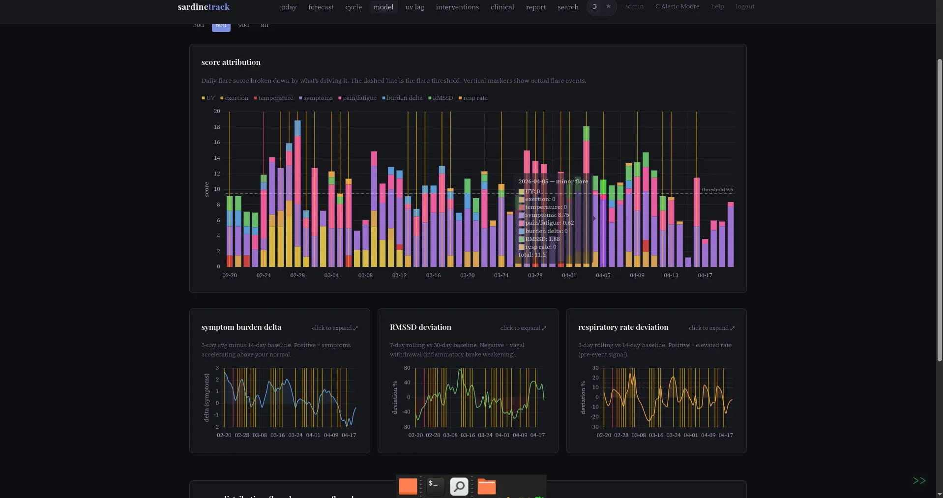
The model dashboard (/timeline, nav label “model”) provides score transparency over time:
- Score attribution chart: Stacked bars showing daily score broken down by component, with flare event markers and threshold line
- Symptom burden delta: Line chart of the baseline-relative delta, showing symptom acceleration
- RMSSD deviation: Line chart showing vagal tone deviation from personal baseline
- Score distribution: Summary statistics comparing flare days vs non-flare days
- Prediction accuracy strip: Per-day colored dots (green = correct, red = missed, orange = false alarm)
RMSSD Trajectory Analysis
The pre-flare pattern analysis page (/forecast/patterns) includes an RMSSD trajectory chart showing the 7 days before each ER visit and major flare:
- Individual event lines (color-coded by severity)
- Aggregate mean line with +/- 1 SD confidence band
- Baseline reference line (non-flare day average)
- Trend direction indicator (rising/falling/flat with magnitude)
This was built to test the hypothesis that RMSSD may behave differently before flares than the simple “vagal withdrawal = drop” model predicts.
Data Sources
| Metric | Source |
|---|---|
| Symptoms, pain, fatigue, emotional state | Manual daily entry |
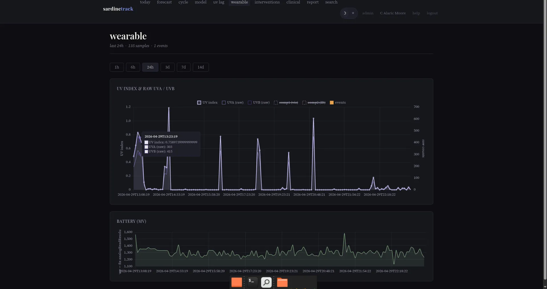
| Steps, HRV (SDNN), resting HR, SpO2, respiratory rate | Apple Watch via iOS health sync app |
| RMSSD | Computed from RR interval heartbeat series (overnight window, 10pm-8am) |
| Basal body temperature | Apple Watch wrist temperature |
| UV index | Open-Meteo and Visual Crossing weather APIs |
| Sun exposure minutes | Manual daily entry |
| Flare events and severity | Manual daily entry |
Relevant Literature
- Huston & Tracey (2011). Cholinergic anti-inflammatory pathway — vagal tone suppresses systemic inflammation via acetylcholine on macrophage nicotinic receptors. Proposed HRV as a predictor of impending relapse. Mechanism behind RMSSD features (sections 7, 7b).
- Thanou A, Stavrakis S, Dyer JW, Munroe ME, James JA, Merrill JT (2016). “Impact of heart rate variability, a marker for cardiac health, on lupus disease activity.” Arthritis Research & Therapy 18:197. Within-subject ΔRMSSD inversely correlated with ΔSLEDAI (p=0.007); LF/HF ratio associated with the SELENA-SLEDAI Flare Index (p=0.008). Direct evidence that RMSSD tracks lupus disease activity longitudinally — core justification for the deviation-based scoring in section 7.
- Poliwczak AR et al. (2017). “The use of heart rate turbulence and heart rate variability in the assessment of autonomic regulation and circadian rhythm in patients with systemic lupus erythematosus without apparent heart disease.” Lupus. 24-hour Holter in 26 SLE women vs 30 controls showing chronic parasympathetic impairment (r-MSSD 23.5 vs 35.7 ms, p=0.002). Establishes that lupus patients have a baseline-reduced RMSSD state even between flares, which is why the features score deviation from personal baseline rather than absolute level.
- Bhatt/Engel group (ACR abstracts). 58 SLE patients, 505 visit pairs. RMSSD and HF-HRV increased during clinical improvement, decreased during flares, inverse correlation to SLEDAI. Supporting evidence alongside Thanou 2016.
- Barfod C et al. (2017). “Abnormal vital signs are strong predictors for intensive care unit admission and in-hospital mortality in adults triaged in the emergency department — a prospective cohort study.” Scandinavian Journal of Trauma, Resuscitation and Emergency Medicine 25:81. General critical-care deterioration literature; OR=1.15 per breath/min increase for 2-day outcome (n=15,724). Non-lupus-specific motivation for the respiratory rate feature in section 8. Honest caveat: not validated in SLE; Alaric’s personal data does not yet confirm the direction.
- Apple Watch HRV validation (2024). Underestimates HRV by ~8.3 ms vs Polar H10 (MAPE ~29%). Tracks relative within-person changes adequately for longitudinal monitoring — the basis for scoring deviation rather than absolute RMSSD.
Built by C. Alaric Moore. Model development and data analysis by Claude Opus (Anthropic) — nicknamed Clode — with statistical validation by a second Claude instance (Wolf).
Installation guide
Excerpted from the project README. Full documentation lives on GitHub.
Requirements
- macOS, Linux, or Windows (tested primarily on macOS and Linux… actually not tested on Windows. Sorry.)
- Python 3.9 or later (earlier veersions work, but watch your D’s and d’s)
- A web browser (Brave, Firefox, Safari, Edge, Opera, Tor…)
- Optional: iPhone with Apple Health for biometric import (I have an apple watch, because access to raw data for free and it’s also a watch)
Installation
Step 1: Install Python
macOS/Linux: Python 3 is likely already installed. Open Terminal and check:
python3 --versionIf you see Python 3.9 or higher, you’re good. If not, download from python.org.
Windows: Download Python from python.org and make sure to check “Add Python to PATH” during installation.
Step 2: Download sardine-track
Option A: Download ZIP (easiest if you’re not familiar with git)
- Go to the GitHub repository page
- Click the green Code button
- Click Download ZIP
- Unzip the file to a folder you can find (like
Documents/sardine-track)
Option B: Clone with git
git clone https://github.com/alaricmoore/sardine-track.git
cd sardine-track
The repo was formerly named
biotracking; the old URL still redirects. If you want the iOS companion as well, the Swift sources live in a separate repo: github.com/alaricmoore/sardinessync.
Step 3: Set Up the Application
Open Terminal (Mac/Linux) or Command Prompt (Windows), navigate to the sardine-track folder, and run:
# Create a virtual environment (recommended)
python3 -m venv .venv

# Activate it
# Mac/Linux:
source .venv/bin/activate
# Windows:
.venv\Scripts\activate

# Install dependencies
pip install -r requirements.txt

# Run first-time setup
python setup.py
The setup script will ask you for:
- Your name (for reports)
- Location coordinates (for UV data — you can find these by Googling “my coordinates” or using latlong.net)
- Timezone (e.g.,
America/Chicago,America/New_York,Europe/London) - Baseline body temperature in Fahrenheit (your normal resting temp, usually around 97-99°F)
Important for coordinates: If you’re in North America, your longitude should be negative. For example, Oklahoma City is
35.4676, -97.5164(note the minus sign on longitude). The setup script will warn you if you forget.
Step 4: Start the Application
python app.pyYou should see:
sardinetrack
============
Patient: Your Name
Starting server...

Local:  http://localhost:5000
Phone:  connect to same wifi, visit http://<your-ip>:5000
A note on the name: internally, the code still calls itself
biotrackingin a lot of places (module docstrings, thebiotracking.dbfilename, some comments). That was the project’s original name before it becamesardine-track. It’s left alone on purpose — renaming every occurrence is churn without benefit, and the database file in particular would break existing installs if renamed. User-facing surfaces (this banner, script output,--helptext) saysardinetrack.
Open your browser and go to http://localhost:5000. Try adding today’s entry to make sure everything works.